A Maximum Likelihood Approach to Continuous Speech Recognition

LALIT R. BAHL, MEMBER, IEEE, FREDERICK JELINEK, FELLOW, IEEE, AND ROBERT L. MERCER

Abstract—Speech recognition is formulated as a problem of maximum likelihood decoding. This formulation requires statistical models of the speech production process. In this paper, we describe a number of statistical models for use in speech recognition. We give special attention to determining the parameters for such models from sparse data. We also describe two decoding methods, one appropriate for constrained artificial languages and one appropriate for more realistic decoding tasks. To illustrate the usefulness of the methods described, we review a number of decoding results that have been obtained with them.

Index Terms—Markov models, maximum likelihood, parameter estimation, speech recognition, statistical models.

[Figure: A continuous speech recognition system.]

Caption: Fig. 1. A continuous speech recognition system. Figure text: TEXT GENERATOR -> SPEAKER -> ACOUSTIC PROCESSOR -> LINGUISTIC DECODER. SPEECH RECOGNIZER.

[Figure: The communication theory view of speech recognition.]

Caption: Fig. 2. The communication theory view of speech recognition. Figure text: TEXT GENERATOR -w-> SPEAKER -> ACOUSTIC PROCESSOR -y-> LINGUISTIC DECODER -w^->. ACOUSTIC CHANNEL.

I. INTRODUCTION

THE AIM of research in automatic speech recognition is the development of a device that transcribes natural speech automatically. Three areas of speech recognition research can be distinguished: 1) isolated word recognition where words are separated by distinct pauses; 2) continuous speech recognition where sentences are produced continuously in a natural manner; and 3) speech understanding where the aim is not transcription but understanding in the sense that the system (e.g., a robot or a database query system) responds correctly to a spoken instruction or request. Commercially available products exist for isolated word recognition with vocabularies of up to several hundred words.

Although this article is confined to continuous speech recognition (CSR), the statistical methods described are applicable to the other two areas of research as well. Acoustics, phonetics, and signal processing are discussed here only as required to provide background for the exposition of statistical methods used in the research carried out at IBM.

Products which recognize continuously spoken small vocabularies are already on the market but the goal of unrestricted continuous speech recognition is far from being realized. All current research is carried out relative to task domains which greatly restrict the sentences that can be uttered. These task domains are of two kinds: those where the allowed sentences are prescribed a priori by a grammar designed by the experimenter (referred to as artificial tasks), and those related to a limited area of natural discourse which the experimenter tries to model from observed data (referred to as natural tasks). Examples of natural tasks are the text of business letters, patent applications, book reviews, etc.

In addition to the constraint imposed by the task domain, the experimental environment is often restricted in several other ways. For example, at IBM speech is recorded with a headset microphone; the system is tuned to a single talker; the talker is prompted by a script, false starts are eliminated, etc.; recognition often requires many seconds of CPU time for each second of speech.

The basic CSR system consists of an acoustic processor (AP) followed by a linguistic decoder (LD) as shown in Fig. 1. Traditionally, the acoustic processor is designed to act as a phonetician, transcribing the speech waveform into a string of phonetic symbols, while the linguistic decoder translates the possibly garbled phonetic string into a string of words. In more recent work [1]–[6], the acoustic processor does not produce a phonetic transcription, but rather produces a string of labels each of which characterizes the speech waveform locally over a short time interval (see Section II).

In Fig. 2, speech recognition is formulated as a problem in communication theory. The speaker and acoustic processor are combined into an acoustic channel, the speaker transforming the text into a speech waveform and the acoustic processor acting as a data transducer and compressor. The channel provides the linguistic decoder with a noisy string from which it must recover the message—in this case the original text. One is free to modify the channel by adjusting the acoustic processor but unlike in communications, one cannot choose the code because it is fixed by the language being spoken. It is possible to allow feedback from the decoder to the acoustic processor but the mathematical consequences of such a step are not well understood. By not including feedback we facilitate a consistent and streamlined formulation of the linguistic decoding problem.

The rest of this article is divided as follows. Section II gives a brief summary of acoustic processing techniques. Section

---

Manuscript received February 23, 1981; revised September 28, 1982. The authors are with the IBM T. J. Watson Research Center, Yorktown Heights, NY 10598.

III formulates the problem of linguistic decoding and shows the necessity of statistical modeling of the text and of the acoustic channel. Section IV introduces Markov models of speech processes. Section V describes an elegant linguistic decoder based on dynamic programming that is practical under certain conditions. Section VI deals with the practical aspects of the sentence hypothesis search conducted by the linguistic decoder. Sections VII and VIII introduce algorithms for extracting model parameter values automatically from data. Section IX discusses methods of assessing the performance of CSR systems, and the relative difficulty of recognition tasks. Finally, in Section X we illustrate the capabilities of current recognition systems by describing the results of certain recognition experiments.

II. ACOUSTIC PROCESSORS

An acoustic processor (AP) acts as a data compressor of the speech waveform. The output of the AP should 1) preserve the information important to recognition and 2) be amenable to statistical characterization. If the AP output can be easily interpreted by people, it is possible to judge the extent to which the AP fulfills requirement 1).

Typically, an AP is a signal processor, which transforms the speech waveform into a string of parameter vectors, followed by a pattern classifier, which transforms the string of parameter vectors into a string of labels from a finite alphabet. If the pattern classifier is absent, then the AP produces an unlabeled string of parameter vectors. In a segmenting AP, the speech waveform is segmented into distinct phonetic events (usually phones¹) and each of these varying length portions is then labeled.

A time-synchronous AP produces parameter vectors computed from successive fixed-length intervals of the speech waveform. The distance from the parameter vector to each of a finite set of standard parameter vectors, or prototypes, is computed. The label for the parameter vector is the name of the prototype to which it is closest.

In early acoustic processors, prototypes were obtained from speech data labeled by an expert phonetician. In more recent acoustic processors, prototypes are obtained automatically from unlabeled speech data [3], [4].

A typical example of a time-synchronous AP is the IBM centisecond acoustic processor (CSAP). The acoustic parameters used by CSAP are the energies in each of 80 frequency bands in steps of 100 Hz covering the range from 0-8000 Hz. They are computed once every centisecond using a 2 cs window. The pattern classifier has 45 prototypes corresponding roughly to the phones of English. Each prototype for a given speaker is obtained from several samples of his speech which has been carefully labeled by a phonetician.

III. LINGUISTIC DECODER

The AP produces an output string y. From this string y, the linguistic decoder (LD) makes an estimate ŵ of the word string w produced by the text generator (see Fig. 1). To minimize the probability of error, ŵ must be chosen so that $$P(\hat{\mathbf{w}}|\mathbf{y}) = \max_{\mathbf{w}} P(\mathbf{w}|\mathbf{y}). \quad (3.1)$$

By Bayes’ rule $$P(\mathbf{w}|\mathbf{y}) = \frac{P(\mathbf{w}) P(\mathbf{y}|\mathbf{w})}{P(\mathbf{y})}. \quad (3.2)$$

Since $P(\mathbf{y})$ does not depend on w, maximizing $P(\mathbf{w}|\mathbf{y})$ is equivalent to maximizing the likelihood $P(\mathbf{w}, \mathbf{y}) = P(\mathbf{w}) P(\mathbf{y}|\mathbf{w})$. Here $P(\mathbf{w})$ is the a priori probability that the word sequence w will be produced by the text generator, and $P(\mathbf{y}|\mathbf{w})$ is the probability with which the acoustic channel (see Fig. 1) transforms the word string w into the AP output string y.

To estimate $P(\mathbf{w})$, the LD requires a probabilistic model of the text generator, which we refer to as the language model. For most artificial tasks, the language modeling problem is quite simple. Often the language is specified by a small finite-state or context-free grammar to which probabilities can be easily attached. For example, the Raleigh language (see Section IV) is specified by Fig. 7 where all words possible at any point are considered equally likely.

For natural tasks the estimation of $P(\mathbf{w})$ is much more difficult. Linguistics has not progressed to the point that it can provide a grammar for a sizable subset of natural English, which is useful for speech recognition. In addition, the interest in linguistics has been in specifying the sentences of a language, but not their probabilities. Our approach has been to model the text generator as a Markov source, the parameters of which are estimated from a large sample of text.

To estimate $P(\mathbf{y}|\mathbf{w})$, the other component of the likelihood, the LD requires a probabilistic model of the acoustic channel, which must account for the speaker’s phonological and acoustic-phonetic variations and for the performance of the acoustic processor. Once models are available for computing $P(\mathbf{w})$ and $P(\mathbf{y}|\mathbf{w})$, it is in principle possible for the LD to compute the likelihood of each sentence in the language and determine the most likely ŵ directly. However, even a small artificial language such as the Raleigh language has several million possible sentences. It is therefore necessary in practice to carry out a suboptimal search. A dynamic programming search algorithm, the applicability of which is limited to tasks of moderate complexity, is described in Section V. A more general tree search decoding algorithm is described in Section VI.

IV. MARKOV SOURCE MODELING OF SPEECH PROCESSES

Notation and Terminology

By a Markov source, we mean a collection of states connected to one another by transitions which produce symbols from a finite alphabet. Each transition $t$ from a state $s$ has associated with it a probability $q_s(t)$ which is the probability that $t$ will be chosen next when $s$ is reached. From the states of a Markov source we choose one state as the initial state and one state as the final state. The Markov source then assigns probabilities to all strings of transitions from the initial state to the final state. Fig. 3 shows an example of a Markov source.

[Figure: A Markov source diagram with states and transitions labeled with 0 and 1]

Caption: Fig. 3. A Markov source.

[Figure: A Markov source diagram with states, transitions, and null transitions represented by dashed lines]

Caption: Fig. 4. A Markov source with null transitions.

[Figure: A block diagram showing a Markov source connected to a filter]

Caption: Fig. 5. A filtered Markov source. Figure text: MARKOV SOURCE; a1, ..., an, ...; FILTER; b1, ..., bm, ...

[Figure: A sequence of transitions labeled t1 through t6 with output symbols b1, b2, b3 and null transitions]

Caption: Fig. 6. A sequence of transitions to illustrate spanning. b1 spans t1; b2 spans t2, t3, t4; and b3 spans t5, t6.

We define a Markov source more formally as follows. Let $\mathcal{S}$ be a finite set of states, $\mathcal{T}$ a finite set of transitions, and $\mathcal{A}$ a finite alphabet. Two elements of $\mathcal{S}$, $s_I$ and $s_F$ are distinguished as initial and final states, respectively. The structure of a Markov source is a 1-1 mapping $M: \mathcal{T} \to \mathcal{S} \times \mathcal{A} \times \mathcal{S}$. If $M(t) = (l, a, r)$ then we refer to $l$ as the predecessor state of $t$, $a$ as the output symbol associated with $t$, and $r$ as the successor state of $t$; we write $l = L(t)$, $a = A(t)$, and $r = R(t)$.

The parameters of a Markov source are probabilities $q_s(t)$, $s \in \mathcal{S} - {s_F}$, $t \in \mathcal{T}$, such that

$q_s(t) = 0 \quad \text{if } s \neq L(t)$

and

$\sum_t q_s(t) = 1, \quad s \in \mathcal{S} - {s_F}$. (4.1)

In general, the transition probabilities associated with one state are different from those associated with another. However, this need not always be the case. We say that state $s_1$ is tied to state $s_2$ if there exists a 1-1 correspondence $T_{s_1s_2}: \mathcal{T} \to \mathcal{T}$ such that $q_{s_1}(t) = q_{s_2}(T_{s_1s_2}(t))$ for all transitions $t$. It is easily verified that the relationship of being tied is an equivalence relation and hence induces a partition of $\mathcal{S}$ into sets of states which are mutually tied.

A string of $n$ transitions $\mathbf{t}_1^n$ for which $L(t_1) = s_I$ is called a path; if $R(t_n) = s_F$, then we refer to it as a complete path. The probability of a path $\mathbf{t}_1^n$ is given by

$P(\mathbf{t}1^n) = q{s_I}(t_1) \prod_{i=2}^n q_{R(t_{i-1})}(t_i).$ (4.2)

Associated with path $\mathbf{t}_1^n$ is an output symbol string $\mathbf{a}_1^n = A(\mathbf{t}_1^n)$. A particular output string $\mathbf{a}_1^n$, may in general arise from more than one path. Thus, the probability $P(\mathbf{a}_1^n)$ is given by

$P(\mathbf{a}1^n) = \sum{\mathbf{t}_1^n} P(\mathbf{t}_1^n) \delta(A(\mathbf{t}_1^n), \mathbf{a}_1^n)$ (4.3)

where

$\delta(a, b) = \begin{cases} 1 & \text{if } a = b \ 0 & \text{otherwise.} \end{cases}$ (4.4)

A Markov source for which each output string $\mathbf{a}_1^n$ determines a unique path is called a unifilar Markov source.

In practice it is useful to allow transitions which produce no output. These null transitions are represented diagrammatically by interrupted lines (see Fig. 4). Rather than deal with null transitions directly, we have found it convenient to associate with them the distinguished letter $\phi$. We then add to the Markov source a filter (see Fig. 5) which removes $\phi$, transforming the output sequence $\mathbf{a}_1^n$ into an observed sequence $\mathbf{b}_1^m$, where $b_i \in \mathcal{B} = \mathcal{A} - {\phi}$. Although more general sources can be handled, we shall restrict our attention to sources which do not have closed circuits of null transitions.

If $\mathbf{t}_1^n$ is a path which produces the observed output sequence $\mathbf{b}_1^m$, then we say that $b_i$ spans $t_j$ if $t_j$ is the transition which produced $b_i$ or if $t_j$ is a null transition immediately preceding a transition spanned by $b_i$. For example, in Fig. 6, $b_1$ spans $t_1$; $b_2$ spans $t_2, t_3, t_4$; and $b_3$ spans $t_5$ and $t_6$.

A major advantage of using Markov source models for the text generator and acoustic channel is that once the structure is specified, the parameters can be estimated automatically from data (see Sections VII and VIII). Furthermore, computationally efficient algorithms exist for computing $P(\mathbf{w})$ and $P(\mathbf{y}|\mathbf{w})$ with such models (see Sections V and VI). Markov source models also allow easy estimation of the relative difficulty of recognition tasks (see Section IX).

The Language Model

Since the language model has to assign probabilities to strings of words, it is natural for its output alphabet to be the vocabulary of the language. However, the output alphabet can include shorter units such as word stems, prefixes, suffixes,

[Figure: Grammar of the Raleigh language.]

Caption: Fig. 7. Grammar of the Raleigh language. Figure text: (The figure contains a complex flow diagram of nodes labeled with words like "bad", "black", "gentle", "great", "primary", "proficient", "quiet", "recognition", "small", "sufficient", "distant", "eager", "kind", "large", "new", "other", "tiny", "tired", "true", "ugly", "active", "democratic", "fair", "little", "practical", "poor", "safe", "short", "strong", "backward", "big", "close", "good", "important", "old", "passive", "rugged", "separate", "useless", "condition", "duration", "general", "private", "sergeant", "train", "village", "division", "part", "period", "power", "time", "street", "war", "matters", "men", "people", "practices", "streets", "treaties", "workers", "actions", "bases", "battles", "commands", "forms", "grounds", "places", "considered", "created", "gove", "liked", "made", "moved", "permitted", "wanted", "changes", "does", "fights", "feels", "goes", "lives", "proposes", "votes", "contributed", "criticized", "disturbed", "forgot", "governed", "had", "showed", "took", "appears", "approves", "drinks", "has", "is", "looks", "takes", "works", "accepted", "applied", "brought", "detected", "found", "outlawed", "rejected", "saved", "ask", "get", "know", "make", "pay", "ran", "survive", "were", "believe", "come", "do", "direct", "follow", "proceed", "seem", "stand", "be", "call", "carry", "control", "have", "think", "try", "turn", "bus", "campaign", "food", "gun", "motion", "name", "radio", "ship", "state", "telephone", "thing", "weapon", "building", "captain", "cause", "city", "country", "letter", "major", "man", "nation", "officer", "report", "thought", "again", "excessively", "least", "majorly", "merely", "mostly", "not", "only", "principally", "properly", "sometimes", "truly", "always", "finally", "frequently", "less", "more", "never", "occasionally", "often", "once", "usually", "rarely", "seldomly", "across", "at", "from", "on", "toward", "under", "against", "for", "in", "into", "through", "to", "around", "before", "during", "over", "past", "with", "about", "after", "among", "between", "by", "without", "approaches", "engineers", "girls", "issues", "locations", "operations", "plans", "problems", "sites", "zones", "airplane", "business", "engine", "machine", "missile", "moment", "order", "product", "use", "year", "capitol", "concern", "cover", "day", "interval", "life", "purpose", "sacrifice", "vehicle", "week", "camps", "fields", "houses", "interests", "methods", "scientists", "services", "soldiers", "systems", "techniques")

etc., from which word sequences can be derived. Fig. 7 is the model of the artificial Raleigh language which has been used in some of our experiments. The output alphabet is the 250-word vocabulary of the language. For diagrammatic convenience, sets of transitions between pairs of states have been replaced by single transitions with an associated list of possible output words.

For natural languages, the structure of the model is not given a priori. However,

$$P(w_1^n) = P(w_1)P(w_2|w_1)P(w_3|w_1^2) \cdots P(w_n|w_1^{n-1})$$ $$= \prod_{k=1}^n P(w_k|w_1^{k-1}) \quad (4.5)$$

and so it is natural to consider structures for which a word string $w_1^{k-1}$ uniquely determines the state of the model. A particularly simple model is the $N$-gram model where the state at time $k-1$ corresponds to the $N-1$ most recent words $w_{k-N+1}, \cdots, w_{k-1}$. This is equivalent to using the approximation

$$P(w_1^n) \cong \prod_{k=1}^n P(w_k|w_{k-N+1}^{k-1}).$$

$N$-gram models are computationally practical only for small values of $N$. In order to reflect longer term memory, the state can be made dependent on a syntactic analysis of the entire past word string $w_1^{k-1}$, as might be obtained from an appropriate grammar of the language.

The Acoustic Channel Model

The AP is deterministic and hence the same waveform will always give rise to the same AP output string. However, for a given word sequence, the speaker can produce a great variety of waveforms resulting in a corresponding variation in the AP output string. Some of the variation arises because there are many different ways to pronounce the same word (this is called phonological variation). Other factors include rate of

[Figure: A word-based Markov subsource.]

Caption: Fig. 8. A word-based Markov subsource.

articulation, talker’s position relative to the microphone, ambient noise, etc.

We will only consider the problem of modeling the acoustic channel for single words. Models for word strings can be constructed by concatenation of these simpler, single word models. Fig. 8 is an example of the structure of a Markov source for a single word. The double arcs represent sets of transitions, one for each symbol in the output alphabet. The straight-line path represents pronunciations of average length, while the transitions above and below can lengthen and shorten the pronunciation, respectively. Since the pronunciation of a word depends on the environment in which it occurs, it may be necessary in practice to make the parameters of the model depend on the phonetic environment provided by the preceding and following words.

Since the same sounds can occur in many different words, portions of one model will be similar to portions of many other models. The number of parameters required to specify all the word models can be reduced by modeling sounds or phones rather than words directly. This leads to a two-level model in which word strings are transformed into phone strings which are then transformed into AP output strings. Using this approach, the acoustic channel model is built up from two components: a set of phonetic subsources, one for each word; and a set of acoustic subsources, one for each phone.

Let $\mathcal{P}$ be the alphabet of phones under consideration. A phonetic subsource for a word is a Markov source with output alphabet $\mathcal{P}$ which specifies the pronunciations possible for the word and assigns a probability to each of them. Fig. 9 shows the structure of a phonetic Markov subsource for the word

[Figure: A phonetic Markov subsource.]

Caption: Fig. 9. A phonetic Markov subsource. Figure text: h, u, v, U, v

[Figure: An acoustic Markov subsource.]

Caption: Fig. 10. An acoustic Markov subsource. Figure text: 1, 2, 3, 4, 5, 6, 7

[Figure: A phone-based Markov source based on the phonetic subsource of Fig. 9.]

Caption: Fig. 11. A phone-based Markov source based on the phonetic subsource of Fig. 9. Figure text: ACOUSTIC SUBSOURCE OF PHONE t, ACOUSTIC SUBSOURCE OF PHONE h, ACOUSTIC SUBSOURCE OF PHONE u, ACOUSTIC SUBSOURCE OF PHONE U, ACOUSTIC SUBSOURCE OF PHONE v

two. The structures of these subsources may be derived by the application of phonological rules to dictionary pronunciations for the words [8].

An acoustic subsource for a phone is a Markov source with output alphabet Y which specifies the possible AP output strings for that phone and assigns a probability to each of them. Fig. 10 shows the structure of an acoustic Markov subsource used with the IBM Centisecond Acoustic Processor.

By replacing each of the transitions in the phonetic subsource by the acoustic subsource for the corresponding phone, we obtain a Markov source model for the acoustic channel. This embedding process is illustrated in Fig. 11.

Whereas the structure of the phonetic subsources can be derived in a principled way from phonological rules, the structures of the word model in Fig. 8 and the phone model in Fig. 9 are fairly arbitrary. Many possible structures seem reasonable; the ones shown here are very simple ones which have been used successfully in recognition experiments.

V. VITERBI LINGUISTIC DECODING

In the preceding section we have shown that acoustic subsources can be embedded in phonetic subsources to produce a model for the acoustic channel. In a similar fashion we can embed acoustic channel word models in the Markov source specifying the language model by replacing each transition by the model of the corresponding word. The resulting Markov source is a model for the entire stochastic process to the left of the linguistic decoder in Fig. 1. Each complete path $t_1^n$ through the model determines a unique word sequence $w = W(t_1^n)$ and a unique AP output string $y_1^m = Y(t_1^n)$ and has the associated probability $P(t_1^n)$. Using well known minimum-cost path-finding algorithms, it is possible to determine for a given AP string $y_1^m$, the complete path $t_1^n$ which maximizes the probability $P(t_1^n)$ subject to the constraint $Y(t_1^n) = y_1^m$. A decoder based on this strategy would then produce as its output $W(t_1^n)$. This decoding strategy is not optimal since it may not maximize the likelihood $P(w, y)$. In fact, for a given pair $w, y$ there are many complete paths $t$ for which $W(t) = w$ and $Y(t) = y$. To minimize the probability of error, one must sum $P(t)$ over all these paths and select the $w$ for which the sum is maximum. Nevertheless, good recognition results have been obtained using this suboptimal decoding strategy [1], [2], [9].

A simple method for finding the most likely path is a dynamic programming scheme [10] called the Viterbi Algorithm [11]. Let $\tau_k(s)$ be the most probable path to state $s$ which produces output $y_1^k$. Let $V_k(s) = P(\tau_k(s))$ denote the probability of the path $\tau_k(s)$. We wish to determine $\tau_m(s_F)$.² Because of the Markov nature of the process, $\tau_k(s)$ can be shown to be an extension of $\tau_{k-1}(s')$ for some $s'$. Therefore, $\tau_k(s)$ and $V_k(s)$ can be computed recursively from $\tau_{k-1}(s)$ and $V_{k-1}(s)$ starting with the boundary conditions $V_0(s_1) = 1$ and $\tau_0(s_1)$ being the null string. Let $C(s, a) = {t | R(t) = s, A(t) = a}$. Then

$$V_k(s) = \max { \max_{t \in C(s, y_k)} V_{k-1}(L(t)) q_{L(t)}(t), \max_{t \in C(s, \phi)} V_k(L(t)) q_{L(t)}(t) }. \quad (5.1)$$

If the maximizing transition $t$ is in $C(s, y_k)$ then $\tau_k(s) = \tau_{k-1}(L(t)) \cdot t$; otherwise $t$ must be in $C(s, \phi)$ and $\tau_k(s) = \tau_k(L(t)) \cdot t$, where $\cdot$ denotes concatenation. Note that in (5.1) $V_k(s)$ depends on $V_k(L(t))$ for $t \in C(s, \phi)$. $V_k(L(t))$ must therefore be computed before $V_k(s)$. Because closed circuits of null loops are not allowed,² it is possible to order the states $s_1, s_2, s_3, \dots$, such that $t \in C(s_k, \phi)$ and $L(t) = s_j$ only if $j < k$. If we then compute $V_k(s_1), V_k(s_2)$, etc., in sequence, the necessary values will always be available when required.

Many shortcuts to reduce the amount of computation and storage are possible and we will briefly mention some of the more useful ones. If logarithms of probabilities are used, no multiplications are necessary and the entire search can be carried out with additions and comparisons only. Computation and storage needs can be reduced by saving for each $k$, only those states having relatively large values of $V_k(s)$. This can be achieved by first computing $V_k(\max) = \max_s V_k(s)$ and then eliminating all states $s$ having $V_k(s) < \Delta V_k(\max)$ where $\Delta$ is an appropriately chosen threshold. This makes the search suboptimal, but in practice there is little or no degradation in performance if the threshold $\Delta$ is chosen with care.

This type of search can be used quite successfully on artificial tasks such as the Raleigh language task, where the number of states is of the order of $10^5$.

In addition to its application to suboptimal decoding, the Viterbi algorithm can be used to align an AP output string $y$ with a known word string $w$, by determining the most likely path $t$ which produces $y$ when $w$ is uttered. The path $t$ specifies a sequence of phones which the algorithm puts into correspondence with the symbols forming the sequence $y$. Inspec-

tion of this alignment allows the experimenter to judge the adequacy of his models and provides an intuitive check on the performance of the AP.

VI. STACK LINGUISTIC DECODING

In the previous section we presented a decoding procedure which finds the most likely complete path t for a given AP output string y. This decoding method is computationally feasible only if the state space is fairly small, as is the case in most artificial tasks. However, in the Laser task (described in Section X), the number of states is of the order of $10^{11}$ which makes the Viterbi search unattractive. Furthermore, the procedure is suboptimal because the word string corresponding to the most likely path t may not be the most likely word string. In this section we present a graph-search decoding method which attempts to find the most likely word string. This method can be used with large state spaces.

Search methods which attempt to find optimal paths through graphs have been used extensively in information theory [12] and in artificial intelligence [13]. Since we are interested in finding the most likely word string, the appropriate graph to search is the word graph generated by the language model. When a complete search of the language model graph is computationally impractical, some heuristic must be used for reducing the computation. Here we describe one specific heuristic method that has been used successfully. To reduce the amount of computation, a left-to-right search starting at the initial state and exploring successively longer paths can be carried out. To carry out this kind of search we need to define a likelihood function which allows us to compare incomplete paths of varying length. An obvious choice may seem to be the probability of uttering the (incomplete) sequence w and producing some initial subsequence of the observed string y, i.e.,

$$\sum_{i=0}^{n} P(w, y_1^i) = P(w) \sum_{i=0}^{n} P(y_1^i | w). \quad (6.1)$$

The first term on the right-hand side is the a priori probability of the word sequence w. The second term, referred to as the acoustic match, is the sum over i of the probability that w produces an initial substring $y_1^i$ of the AP output string y. Unfortunately, the value of (6.1) will decrease with lengthening word sequences w, making it unsuitable for comparing incomplete paths of different lengths. Some form of normalization to account for different path lengths is needed. As in the Fano metric used for sequential decoding [12], it is advantageous to have a likelihood function which increases slowly along the most likely path, and decreases along other paths. This can be accomplished by a likelihood function of the form

$$\Lambda(w) = \sum_{i=0}^{n} P(w, y_1^i) \alpha^{n-i} \sum_{w'} P(w', y_{i+1}^n | w, y_1^i). \quad (6.2)$$

If we consider $P(w, y_1^i)$ to be the cost associated with accounting for the initial part of the AP string $y_1^i$ by the word string w, then $\sum_{w'} P(w', y_{i+1}^n | w, y_1^i)$ represents the expected cost of accounting for the remainder of the AP string $y_{i+1}^n$ with some continuation w' of w. The normalizing factor $\alpha$ can be varied to control the average rate of growth of $\Lambda(w)$ along the most likely path. In practice, $\alpha$ can be chosen by trial and error.

An accurate estimate of $\sum_{w'} P(w', y_{i+1}^n | w, y_1^i)$ is, of course, impossible in practice, but we can approximate it by ignoring the dependence on w. An estimate of $E(y_{i+1}^n | y_1^i)$, the average value of $P(w', y_{i+1}^n | y_1^i)$, can be obtained from training data. In practice, a Markov-type approximation of the form

$$E(y_{i+1}^n | y_1^i) = \prod_{j=i+1}^{n} E(y_j | y_{j-k}^{j-1}) \quad (6.3)$$

can be used. Using $k = 1$ is usually adequate.

The likelihood used for incomplete paths during the search is then given by

$$\Lambda(w) = P(w) \sum_{i=0}^{n} P(y_1^i | w) \alpha^{n-i} E(y_{i+1}^n | y_1^i). \quad (6.4)$$

For complete paths, the likelihood is

$$\Lambda(w) = P(w) P(y_1^n | w), \quad (6.5)$$

i.e., the probability that w was uttered and produced the complete output string $y_1^n$.

The likelihood of a successor path $w^k = w^{k-1} w_k$ can be computed incrementally from the likelihood of its immediate predecessor $w^{k-1}$. The a priori probability $P(w^k)$ is easily obtained from the language model using the recursion

$$P(w^k) = P(w^{k-1}) P(w_k | w^{k-1}). \quad (6.6)$$

The acoustic match values $P(y_1^i | w^k)$ can be computed incrementally if the values $P(y_1^i | w^{k-1})$ have been saved [14].

A search based on this likelihood function is easily implemented by having a stack in which entries of the form $(w, \Lambda(w))$ are stored. The stack, ordered by decreasing values of $\Lambda(w)$, initially contains a single entry corresponding to the initial state of the language model. The term stack as used here refers to an ordered list in which entries can be inserted at any position. At each iteration of the search, the top stack entry is examined. If it is an incomplete path, the extensions of this path are evaluated and inserted in the stack. If the top path is a complete path, the search terminates with the path at the top of the stack being the decoded path.

Since the search is not exhaustive, it is possible that the decoded sentence is not the most likely one. A poorly articulated word resulting in a poor acoustic match, or the occurrence of a word with low a priori probability can cause the local likelihood of the most likely path to fall, which may then result in the path being prematurely abandoned. In particular, short function words like the, a, and of, are often poorly articulated, causing the likelihood to fall. At each iteration, all paths having likelihood within a threshold $\Delta$ of the maximum likelihood path in the stack are extended. The probability of prematurely abandoning the most likely path depends strongly on the choice of $\Delta$ which controls the width of the search. Smaller values of $\Delta$ will decrease the amount of search at the expense of having a higher probability of not finding the most likely path. In practice, $\Delta$ can be adjusted by trial and error to give a satisfactory balance between recognition accuracy and computation time. More complicated likelihood functions and

extension strategies have also been used but they are beyond the scope of this paper.

VII. AUTOMATIC ESTIMATION OF MARKOV SOURCE PARAMETERS FROM DATA

Let $P_i(t, b_1^m)$ be the joint probability that $b_1^m$ is observed at the output of a filtered Markov source and that the $i$th output $b_i$ spans $t$.²

The count

$$c(t, b_1^m) \triangleq \sum_{i=1}^m P_i(t, b_1^m)/P(b_1^m) \quad (7.1)$$

is the Bayes a posteriori estimate of the number of times that the transition $t$ is used when the string $b_1^m$ is produced. If the counts are normalized so that the total count for transitions from a given state is 1, then it is reasonable to expect that the resulting relative frequency

$$f_s(t, b_1^m) \triangleq \frac{c(t, b_1^m) \delta(s, L(t))}{\sum_{t'} c(t', b_1^m) \delta(s, L(t'))} \quad (7.2)$$

will approach the transition probability $q_s(t)$ as $m$ increases.

This suggests the following iterative procedure for obtaining estimates of $q_s(t)$.

1. Make initial guesses $q_s^0(t)$.
2. Set $j = 0$.
3. Compute $P_i(t, b_1^m)$ for all $i$ and $t$ based on $q_s^j(t)$.
4. Compute $f_s(t, b_1^m)$ and obtain new estimates $q_s^{j+1}(t) = f_s(t, b_1^m)$.
5. Set $j = j + 1$.
6. Repeat from 3.

To apply this procedure, we need a simple method for computing $P_i(t, b_1^m)$. Now $P_i(t, b_1^m)$ is just the probability that a string of transitions ending in $L(t)$ will produce the observed sequence $b_1^{i-1}$, times the probability that $t$ will be taken once $L(t)$ is reached, times the probability that a string of transitions starting with $R(t)$ will produce the remainder of the observed sequence. If $A(t) = \phi$, then the remainder of the observed sequence is $b_{i+1}^m$, if $A(t) \neq \phi$ then, of course, $A(t) = b_i$ and the remainder of the observed sequence is $b_{i+1}^m$. Thus if $\alpha_i(s)$ denotes the probability of producing the observed sequence $b_1^i$ by a sequence of transitions ending in the state $s$, and $\beta_i(s)$ denotes the probability of producing the observed sequence $b_{i+1}^m$ by a string of transitions starting from the state $s$, then

$$P_i(t, b_1^m) = \begin{cases} \alpha_{i-1}(L(t)) q_{L(t)}(t) \beta_i(R(t)) & \text{if } A(t) = \phi \ \alpha_{i-1}(L(t)) q_{L(t)}(t) \beta_{i+1}(R(t)) & \text{if } A(t) = b_i. \end{cases} \quad (7.3)$$

The probabilities $\alpha_i(s)$ satisfy the equation [15]

$$\alpha_0(s) = \delta(s, s_I) + \sum_t \alpha_0(L(t)) \gamma(t, s, \phi) \quad (7.4a)$$

$$\alpha_i(s) = \sum_t \alpha_{i-1}(L(t)) \gamma(t, s, b_i) + \sum_t \alpha_i(L(t)) \gamma(t, s, \phi) \quad i \ge 1 \quad (7.4b)$$

where

$$\gamma(t, s, a) = q_{L(t)}(t) \delta(R(t), s) \delta(A(t), a). \quad (7.5)$$

As with the Viterbi algorithm described in Section V, the absence of null circuits guarantees that the states can be ordered so that $\alpha_i(s_j)$ may be determined from $\alpha_{i-1}(s), s \in S$, and $\alpha_i(s_k), k < j$.

The probabilities $\beta_i(s)$ satisfy the equations

$$\beta_m(s_F) = 1 \quad (7.6a)$$

$$\beta_i(s) = \sum_t \beta_i(R(t)) \gamma(t, s, \phi) + \sum_t \beta_{i+1}(R(t)) \gamma(t, s, b_i) \quad i \le m, s \neq s_F \quad (7.6b)$$

where $\beta_{m+1}(s) = 0$ and

$$\gamma(t, s, a) = q_{L(t)}(t) \delta(R(t), s) \delta(A(t), a). \quad (7.7)$$

Step 3) of the iterative procedure above then consists of computing $\alpha_i$ in a forward pass over the data, $\beta_i$ in a backward pass over the data, and finally $P_i(t, b_1^m)$ from (7.3). We refer to the iterative procedure together with the method described for computing $P_i(t, b_1^m)$ as the Forward-Backward Algorithm.

The probability, $P(b_1^m)$, of the observed sequence $b_1^m$ is a function of the probabilities $q_s(t)$. To display this dependence explicitly, we write $P(b_1^m, q_s(t))$. Baum [16] has proven that $P(b_1^m, q_s^{j+1}(t)) \ge P(b_1^m, q_s^j(t))$ with equality only if $q_s^j(t)$ is a stationary point (extremum or inflexion point) of $P(b_1^m, \cdot)$. This result also holds if the transition distributions of some of the states are known and hence held fixed or if some of the states are tied³ to one another thereby reducing the number of independent transition distributions.

When applied to a Markov source language model based on $N$-grams as described in Section IV the Forward-Backward Algorithm reduces simply to counting the number of times $K(w|w_1^{N-1})$, that $w$ follows the sequence $w_1^{N-1}$, and setting

$$q_{w_1^{N-1}}(w) = \frac{K(w|w_1^{N-1})}{\sum_w K(w|w_1^{N-1})}. \quad (7.8)$$

This is equivalent to maximum likelihood estimation of the transition probabilities.

When applied to a Markov source model for the acoustic channel, the Forward-Backward Algorithm is more interesting. Let us first consider the word-based channel model indicated in Fig. 8. A known text $w_1^n$ is read by the speaker and processed by the acoustic processor to produce an output string $y_1^m$. The Markov source corresponding to the text is constructed from the subsources for the words with the assumption that states of the source which arise from the same subsource state are tied. The Forward-Backward Algorithm then is used to estimate the transition probabilities of the subsources from the output string $y_1^m$. To obtain reliable estimates of the subsource transition probabilities, it is necessary that each word in the vocabulary occur sufficiently often in

the text $w_1^n$. For large vocabularies this may require an exorbitant amount of reading.

The use of the phone-based model shown in Fig. 10 can overcome this problem. The Markov source for the text is constructed from phonetic and acoustic subsources as described in Section IV. States in the source arising from the same acoustic subsource state are assumed to be tied. In addition, states from different phonetic subsources are assumed to be tied if transitions leaving the states result from the same phonological rules. With these assumptions the training text can be considerably shorter since it need only include sufficiently many instances of each phone and each phonetic rule.

VIII. PARAMETER ESTIMATION FROM INSUFFICIENT DATA

It is often the case in practice that the data available are insufficient for a reliable determination of all of the parameters of a Markov model. For example, the trigram model for the Laser Patent Text corpus [18] used at IBM Research is based on 1.5 million words. Trigrams which do not occur among these 1.5 million words are assigned zero probability by maximum likelihood estimation, a degenerate case of the Forward-Backward Algorithm. Even though each of these trigrams is very improbable, there are so many of them that they constitute 23 percent of the trigrams present in new samples of text. In other words, after looking at 1.5 million trigrams the probability that the next one seen will never have been seen before is roughly 0.23. The Forward-Backward Algorithm provides an adequate probabilistic characterization of the training data but the characterization may be poor for new data. A method for handling this problem, presented in detail in [15], is discussed in this section.

Consider a Markov source model the parameters of which are to be estimated from data $b_1^m$. We assume that $b_1^m$ is insufficient for the reliable estimation of all of the parameters.

Let $\hat{q}_s(t)$ be forward-backward estimates of the transition probabilities based on $b_1^m$ and let $^\hat{q}_s(t)$ be the corresponding estimates obtained when certain of the states are assumed to be tied. Where the estimates $\hat{q}_s(t)$ are unreliable, we would like to fall back to the more reliably estimated $^\hat{q}_s(t)$, but where $\hat{q}_s(t)$ is reliable we would like to use it directly.

A convenient way to achieve this is to choose as final estimates of $q_s(t)$ a linear combination of $\hat{q}_s(t)$ and $^*\hat{q}_s(t)$. Thus we let $\tilde{q}_s(t)$ be given by

$$\tilde{q}_s(t) = \lambda_s \hat{q}_s(t) + (1 - \lambda_s) ^*\hat{q}_s(t) \quad (8.1)$$

with $\lambda_s$ chosen close to 1 when $\hat{q}_s(t)$ is reliable and close to 0 when it is not.

Fig. 12(a) shows the part of the transition structure of the Markov source related to the state $s$. Equation (8.1) can be interpreted in terms of the associated Markov source shown in Fig. 12(b), in which each state is replaced by three states. In Fig. 12(b), $\hat{s}$ corresponds directly to $s$ in Fig. 12(a). The null transitions from $\hat{s}$ to $s$ and $s^$ have transition probabilities equal to $\lambda_s$ and $1 - \lambda_s$, respectively. The transitions out of $s$ have probabilities $q_s(t) = \hat{q}_s(t)$ while those out of $s^$ have probabilities $^q_s(t) = ^\hat{q}_s(t)$. The structure of the associated Markov source is completely determined by the structure of the original Markov source and by the tyings assumed for obtaining more reliable parameter estimates.

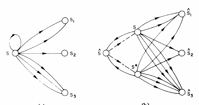
Caption: Fig. 12. (a) Part of transition structure of a Markov source. (b) The corresponding part of an associated interpolated Markov source. Figure text: (a) S, S1, S2, S3. (b) S, S1, S*, S2, S3.

The interpretation of (8.1) as an associated Markov source immediately suggests that the parameters $\lambda_s$ be determined by the Forward-Backward (FB) Algorithm. However, since the $\lambda$ parameters were introduced to predict as yet unseen data, rather than to account for the training data $b_1^m$, the FB Algorithm must be modified. We wish to extract the $\lambda$ values from data that was not used to determine the distributions $\hat{q}_s(t)$ and $^\hat{q}_s(t)$ [see (8.1)]. Since presumably we have only $b_1^m$ at our disposal, we will proceed by the deleted interpolation method. We shall divide $b_1^m$ into $n$ blocks and for $i = 1, \cdots, n$ estimate $\lambda$ from the $i$th block while using $\hat{q}_s(t)$ and $^\hat{q}_s(t)$ estimates derived from the remaining blocks.

Since the $\lambda_s$ values should depend on the reliability of the estimate $\hat{q}_s(t)$, it is natural to associate them with the estimated relative frequency of occurrence of the state $s$. We thus decide on $k$ relative frequency ranges and aim to determine corresponding values $\lambda(1), \cdots, \lambda(k)$. Then $\lambda_s = \lambda(i)$ if the relative frequency of $s$ was estimated to fall within the $i$th range.

We partition the state space $S$ into subsets of tied states $S_1^, S_2^, \cdots, S_r^$ and determine the transition correspondence functions $T_{s,s'}$ for all pairs of tied states $s, s'$. We recall from Section IV that then $^\hat{q}s(t) = ^*\hat{q}{s'}(T_{s,s'}(t))$ for all pairs $s, s' \in S_i^, i = 1, \cdots, r$. If $L(t) \in S_i^$, then $\mathcal{T}(t) = {t' | t' = T_{L(t),s'}(t), s' \in S_i^*}$ is the set of transitions that are tied to $t$. Since $T_{L(t),L(t)}(t) = t$, then $t \in \mathcal{T}(t)$.

We divide the data $b_1^m$ into $n$ blocks of length $l$ ($m = nl$). We run the FB Algorithm in the ordinary way, but on the last iteration we establish separate counters

$$c_j(t, b_1^m) \triangleq \sum_{i=1}^{(j-1)l} P_i(t, b_1^m) + \sum_{i=jl+1}^{m} P_i(t, b_1^m) \quad (8.2)$$

$$j = 1, 2, \cdots, n$$

for each deleted block of data. The above values will give rise to detailed distributions

$$q_s(t, j) = \frac{c_j(t, b_1^m) \delta(s, L(t))}{\sum_{t'} c_j(t', b_1^m) \delta(s, L(t'))} \quad (8.3)$$

and to tied distributions

$$^*q_s(t) = \frac{\delta(s, L(t)) \sum_{t' \in \mathcal{T}(t)} c_j(t', b_1^m)}{\sum_{t'} \delta(s, L(t')) \sum_{t'' \in \mathcal{T}(t')} c_j(t'', b_1^m)} \quad (8.4)$$

Note that $q_s(t, j)$ and $^*q_s(t, j)$ do not depend directly on the output data belonging to the $j$th block. Thus the data in the $j$th block can be considered new in relation to these probabilities.

We now run the FB Algorithm on data $b_j^m$ to determine the $\lambda$ values based on $n$ associated Markov sources which have fixed distributions over transitions leaving the states $s$ and $s^*$. These $\lambda$ values are obtained from estimates of probabilities of transitions leaving the states $\hat{s}$ of the associated Markov source [see Fig. 12(b)]. Only $k$ counter pairs pertaining to the values $\lambda(i)$ and $1 - \lambda(i)$ being estimated are established. When running on the data of the $j$th block, the $j$th associated Markov source is used based on the probabilities $q_s(t, j)$ and $^*q_s(t, j)$. The values $\lambda_s$ used in the $j$th block are chosen by computing the frequency estimates

$$q(s, j) = \frac{\sum_t c_j(t, b_j^m) \delta(s, L(t))}{\sum_{t'} c_j(t', b_j^m)}$$ (8.5)

and setting $\lambda_s = \lambda(i)$ if $q(s, j)$ belonged to the $i$th frequency range. Also, the $\lambda_s$ counts estimated from the $j$th block are then added to the contents of the $i$th counter pair.

After $\lambda$ values have been computed, new test data is predicted using an associated Markov source based on probabilities

$$q_s(t) = \frac{\delta(s, L(t)) \sum_{j=1}^n c_j(t, b_j^m)}{\sum_{t'} \delta(s, L(t')) \sum_{j=1}^n c_j(t', b_j^m)}$$ (8.6)

$$^*q_s(t) = \frac{\delta(s, L(t)) \sum_{t' \in \mathcal{T}(t)} \sum_{j=1}^n c_j(t', b_j^m)}{\sum_{t'} \delta(s, L(t')) \sum_{t'' \in \mathcal{T}(t')} \sum_{j=1}^n c_j(t'', b_j^m)}$$ (8.7)

and $\lambda_s$ values chosen from the derived set $\lambda(1), \dots, \lambda(k)$, depending on the range within which the estimate

$$q(s) = \frac{\sum_t \delta(s, L(t)) \sum_{j=1}^n c_j(t, b_j^m)}{\sum_{t'} \sum_{j=1}^n c_j(t', b_j^m)}$$ (8.8)

falls. It might appear that the convergence of the estimation of the interpolation weights $\lambda(i)$ needs proving since it involves the use of different fixed distributions $q(s, j)$ over different blocks $j = 1, \dots, n$. However, some thought will reveal that the problem can be reformulated in terms of a single more complex Markov source, some of whose parameters are tied and others fixed. This source is identical to the trellis that is needed to carry out the $\lambda$ estimation. The process consists of carrying out the Forward-Backward Algorithms for estimating the parameters of the complex Markov source, and thus converges by the Baum theorem [16].

This approach to modeling data generation is called deleted interpolation. Several variations are possible some of which

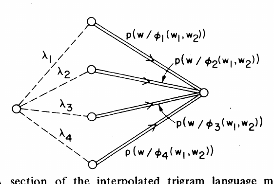
Caption: Fig. 13. A section of the interpolated trigram language model corresponding to the state determined by the word pair $w_1, w_2$. Figure text: $\lambda_1$, $\lambda_2$, $\lambda_3$, $\lambda_4$, $p(w/\phi_1(w_1, w_2))$, $p(w/\phi_2(w_1, w_2))$, $p(w/\phi_3(w_1, w_2))$, $p(w/\phi_4(w_1, w_2))$

are described in [15]. In particular, it is possible to have $v$ different tying partitions of the state space corresponding to transition distributions $^{(i)}q_s(t), i = 1, \dots, v$, and to obtain the final estimates by the formula

$$\tilde{q}s(t) = \sum{i=1}^v \lambda_i(s) ^{(i)}q_s(t)$$ (8.9)

with $\lambda_i(s)$ values determined by the Forward-Backward Algorithm.

We illustrate this deleted interpolation algorithm with an application to the trigram language model for the laser patent text corpus used at IBM.

Let $\pi(w)$ be the syntactic part of speech (e.g., noun, verb, etc.) assigned to the word $w$. Let $\phi_i, i = 1, \dots, 4$ be functions classifying the language model states $w_1 w_2$ as follows:

$$\phi_1(w_1 w_2) = {(w_1 w_2)}$$ $$\phi_2(w_1 w_2) = {(ww_2) | \pi(w) = \pi(w_1)}$$ $$\phi_3(w_1 w_2) = {(ww') | \pi(w) = \pi(w_1), \pi(w') = \pi(w_2)}$$ $$\phi_4(w_1 w_2) = {\text{all pairs of words}}.$$ (8.10)

Let $K(\phi_i(w_1 w_2))$ be the number of times that members of the set $\phi_i(w_1 w_2)$ occur in the training text. Finally, partition the state space into sets

$$\phi_5(w_1 w_2) = {ww' | K(\phi_i(ww')) = K(\phi_i(w_1 w_2)) = 1$$ $$j = 1, 2, \dots, i - 1,$$ $$K(\phi_i(ww')) = K(\phi_i(w_1 w_2)) > 1}$$ (8.11)

which will be used to tie the associated states $w_1 w_2$ according to the frequency of word pair occurrence. Note that if $K(\phi_i(w_1 w_2)) \ge 2$, then $\phi_5(w_1 w_2)$ is simply the set of all word pairs that occurred in the corpus exactly as many times as $w_1 w_2$ did. A different $\lambda$ distribution will correspond to each different set (8.11). The language model transition probabilities are given by the formula

$$\hat{P}(w_3 | w_1 w_2) = \sum_{i=1}^4 \lambda_i(\phi_5(w_1 w_2)) P_i(w_3 | \phi_i(w_1 w_2)).$$ (8.12)

Fig. 13 illustrates this graphically. We use deleted interpolation also in estimating the probabilities associated with the acoustic channel model.

IX. A MEASURE OF DIFFICULTY FOR FINITE STATE RECOGNITION TASKS

Research in continuous speech recognition has led to the development of a number of artificial tasks. In order to compare the performance of different systems on sentences from different tasks, it is necessary to have a measure of the intrinsic difficulty of a task. Although vocabulary size is almost always mentioned in the description of an artificial task, by itself it is practically useless as a measure of difficulty. In this section we describe perplexity, a measure of difficulty based on well established information theoretic principles. The experimental results described in the next section show a clear correlation between increasing perplexity and increasing error rate.

Perplexity is defined in terms of the information theoretic concept of entropy. The tasks used in speech recognition can be adequately modeled as unifilar⁴ Markov sources. Let $P(w|s)$ be the probability that word $w$ will be produced next when the current state is $s$. The entropy, $H_s(w)$ associated with state $s$ is

$H_s(w) = - \sum_{w} P(w|s) \log_2 P(w|s).$ (9.1)

The entropy $H(w)$ of the task is simply the average value of $H_s(w)$. Thus if $\pi(s)$ is the probability of being in state $s$ during the production of a sentence, then

$H(w) = \sum_{s} \pi(s) H_s(w).$ (9.2)

The perplexity $S(w)$ of the task is given in terms of its entropy $H(w)$ by

$S(w) = 2^{H(w)}.$ (9.3)

Often, artificially constrained tasks specify the sentences possible without attaching probabilities to them. Although the task perplexity depends on the probabilities assigned to the sentences, Shannon [17] has shown that the maximum entropy achievable for a task with $N$ possible sentences of average length $l$ is $1/l \log_2 N$. Hence the maximum perplexity is $N^{1/l}$. If all the sentences for the task could be arranged as a regular tree, the number of branches emanating from a node would be $N^{1/l}$. So, for artificially constrained tasks, perplexity can be thought of as the average number of alternative words at each point. For the Raleigh task of Fig. 7, the number of alternative words ranges from 1 to 24, and the perplexity is 7.27.

For natural language tasks, some sentences are much more probable than others and so the maximum perplexity is not useful as a measure of difficulty. However, the perplexity, which can be computed from the probabilities of the sentences, remains a useful measure. Information theory shows that for a language with entropy $H$, we can ignore all but the most probable $2^{lH}$ strings of length $l$ and still achieve any prescribed error rate.

The definition of perplexity makes no use of the phonetic character of the words in the vocabulary of the language. Two tasks may have the same perplexity but one may have words that are substantially longer than the other, thereby making recognition easier. This problem can be overcome by considering the sentences of the task to be strings of phonemes rather than strings of words. We can then compute the phoneme level perplexity of the two tasks and normalize them to words of equal length. In this way the perplexity of the task with the greater average word length will be lowered relative to that of the other task.

Some pairs of phonemes are more confusable than others. It is possible therefore to have two tasks with the same phoneme level perplexity, one of which is much easier to recognize than the other, simply because its words are acoustically farther apart. We can take this into account by considering the joint probability distribution $P(\mathbf{w}, \mathbf{y})$ of word sequences $\mathbf{w}$ and acoustic sequences $\mathbf{y}$ and determining from it the conditional entropy $H(\mathbf{w}|\mathbf{y})$. $\mathbf{y}$ could be the output string from a particular acoustic processor or simply the time waveform itself. Unfortunately, this is far too difficult to compute in practice.

Perplexity reflects the difficulty of recognition when a complete search can be performed. The effect on the error rate of performing an incomplete search may be more severe for one language than for another, even though they have the same perplexity. However, as the results in the next section show, there is a clear correlation between perplexity and error rate.

The results given in this section, obtained before 1980, are described in detail in [3], [5], [6], [18], [19].

Table I shows the effect of training set size of recognition error rate. 200 sentences from the Raleigh Language (100 training and 100 test) were recognized using a segmenting acoustic processor and a stack algorithm decoder. We initially estimated the acoustic channel model parameters by examining samples of acoustic processor output. These parameter values were then refined by applying the Forward-Backward Algorithm to training sets of increasing size. While for small training set sizes performance on training sentences should be substantially better than on test sentences, for sufficiently large training set sizes performance on training and text sentences should be about equal. By this criterion a training set size of 600 sentences is adequate for determining the parameters of this acoustic channel model. Notice that even a training set size as small as 200 sentences leads to a substantial reduction in error rate as compared to decoding with the initially estimated channel model parameters.

The power of automatic training is evident from Table I in the dramatic decrease in error rate resulting from training even with a small amount of data. The results in Table II further demonstrate the power of automatic training. Here, three versions of the acoustic channel model are used, each weaker than the previous one. The "complete acoustic channel model" result corresponds to the last line of Table I. The acoustic channel model in this case is built up from phonetic subsources and acoustic subsources as described in Section IV. The phonetic subsources produce many different strings for each word reflecting phonological modifications due to rate of articulation, dialect, etc. The "single pronunciation" result is obtained with an acoustic channel model in which the phonetic subsources allow only a single pronunciation for each word. Finally, the "spelling-based pronunciation" result is obtained with an

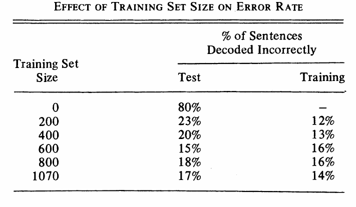
Caption: TABLE I EFFECT OF TRAINING SET SIZE ON ERROR RATE Figure text: Training Set Size | % of Sentences Decoded Incorrectly | Test | Training | 0 | 80% | - | 200 | 23% | 12% | 400 | 20% | 13% | 600 | 15% | 16% | 800 | 18% | 16% | 1070 | 17% | 14%

[Figure: Table II Effect of Weak Acoustics Channel Models and Table III Decoding Results for Several Different Acoustic Processors with the Raleigh Language]

Caption: TABLE II EFFECT OF WEAK ACOUSTICS CHANNEL MODELS TABLE III DECODING RESULTS FOR SEVERAL DIFFERENT ACOUSTIC PROCESSORS WITH THE RALEIGH LANGUAGE Figure text: TABLE II: Model Type | % of Sentences Decoded Incorrectly | Complete Acoustic Channel Model | 17% | Single Pronounciation | 25% | Spelling-Based Pronounciation | 57% | TABLE III: Acoustic Processor | Error Rate | Sentence | Word | MAP | 27% | 3.6% | CSAP | 2% | 0.2% | TRIVIAL | 2% | 0.2%

[Figure: Table IV Recognition Results for Several Tasks of Varying Perplexity]

Caption: TABLE IV RECOGNITION RESULTS FOR SEVERAL TASKS OF VARYING PERPLEXITY Figure text: Vocabulary | Word Error Rate | Task | Size | Perplexity | Segmenting AP | Time-Synchronous AP | CMU-AIX05 | 1011 | 4.53 | 0.8% | 0.1% | Raleigh | 250 | 7.27 | 3.1% | 0.6% | Laser | 1000 | 24.13 | 33.1% | 8.9%

acoustic channel model in which the single pronunciation allowed by the phonetic subsources is based directly on the letter-by-letter spelling of the word. This leads to absurd pronunciation models for some of the words. For example, through is modeled as if the final g and h were pronounced. The trained parameters for the acoustic channel with spelling-based pronunciations show that letters are often deleted by the acoustic processor reflecting the large number of silent letters in English spelling. Although the results obtained in this way are much worse than those obtained with the other two channel models, they are still considerably better than the results obtained with the complete channel model using parameters estimated by people.

Table III shows results on the Raleigh Language for several different acoustic processors. In each case the same set of 100 sentences was decoded using the stack decoding algorithm. MAP is a segmenting acoustic processor, while CSAP and TRIVIAL are nonsegmenting acoustic processors. Prototypes for CSAP were selected by hand from an examination of speech data. Those for TRIVIAL were obtained automatically from a Viterbi alignment of about one hour of speech data.

Table IV summarizes the performance of the stack decoding algorithm with a segmenting and a time-synchronous acoustic processor on three tasks of varying perplexity. The Raleigh task has been described earlier in the paper. The Laser task is a natural language task used at IBM. It consists of sentences from the text of patents in laser technology. To limit the vocabulary, only sentences made entirely from the 1000 most frequent words in the complete laser corpus are considered. The CMU-AIX05 task [20] is the task used by Carnegie-Mellon University in their Speech Understanding System to meet the ARPA specifications [21]. All these results were obtained with sentences spoken by a single talker in a sound-treated room. Approximately 1000 sentences were used for estimating the parameters of the acoustic channel model in each of the experiments. There is a clear correlation between perplexity and error rate. The CMU-AIX05 task has the largest vocabulary but the smallest perplexity. Note that for each of the tasks, the performance of the time-synchronous acoustic processor is considerably better than that of the segmenting acoustic processor.

ACKNOWLEDGMENT

We would like to acknowledge the contributions of the following present and past members of the Continuous Speech Recognition Group at the IBM Thomas J. Watson Research

Center: J. K. Baker, J. M. Baker, R. Bakis, P. Cohen, A. Cole, R. Dixon, B. Lewis, E. Muckstein, and H. Silverman.

REFERENCES

[1] R. Bakis, "Continuous speech recognition via centisecond acoustic states," presented at the 91st Meeting Acoust. Soc. Amer., Washington, DC, Apr. 1976; also IBM Res. Rep. RC-5971, IBM Res. Center, Yorktown Heights, NY, Apr. 1976.

[2] B. T. Lowerre, "The Harpy speech recognition system," Ph.D. dissertation, Dep. Comput. Sci., Carnegie-Mellon Univ., Pittsburgh, PA, 1976.

[3] L. R. Bahl, R. Bakis, P. S. Cohen, A. G. Cole, F. Jelinek, B. L. Lewis, and R. L. Mercer, "Recognition results with several acoustic processors," in Proc. IEEE Int. Conf. Acoust., Speech, Signal Processing, Washington, DC, Apr. 1979, pp. 249-251.

[4] J. M. Baker, "Performance statistics of the hear acoustic processor," in Proc. IEEE Int. Conf. Acoust., Speech, Signal Processing, Washington, DC, Apr. 1979, pp. 262-265.

[5] L. R. Bahl, J. K. Baker, P. S. Cohen, N. R. Dixon, F. Jelinek, R. L. Mercer, and H. F. Silverman, "Preliminary results on the performance of a system for the automatic recognition of continuous speech," in Proc. IEEE Int. Conf. Acoust., Speech, Signal Processing, Philadelphia, PA, Apr. 1976, pp. 425-429.

[6] L. R. Bahl, J. K. Baker, P. S. Cohen, A. G. Cole, F. Jelinek, B. L. Lewis, and R. L. Mercer, "Automatic recognition of continuously spoken sentences from a finite state grammar," in Proc. IEEE Int. Conf. Acoust., Speech, Signal Processing, Tulsa, OK, Apr. 1978, pp. 418-421.

[7] J. Lyons, Introduction to Theoretical Linguistics. Cambridge, England: Cambridge Univ. Press, 1969.

[8] P. S. Cohen and R. L. Mercer, "The phonological component of an automatic speech-recognition system," in Speech Recognition, D. R. Reddy, Ed. New York: Academic, 1975, pp. 275-320.

[9] J. K. Baker, "The DRAGON system—An overview," IEEE Trans. Acoust., Speech, Signal Processing, vol. ASSP-23, pp. 24-29, Feb. 1975.

[10] R. E. Bellman, Dynamic Programming. Princeton, NJ: Princeton Univ. Press, 1957.

[11] G. D. Forney, Jr., "The Viterbi algorithm," Proc. IEEE, vol. 61, pp. 268-278, Mar. 1973.

[12] F. Jelinek, "A fast sequential decoding algorithm using a stack," IBM J. Res. Develop., vol. 13, pp. 675-685, Nov. 1969.

[13] N. J. Nilsson, Problem-Solving Methods in Artificial Intelligence. New York: McGraw-Hill, 1971.

[14] L. R. Bahl and F. Jelinek, "Decoding for channels with insertions, deletions, and substitutions with applications to speech recognition," IEEE Trans. Inform. Theory, vol. IT-21, pp. 404-411, July 1975.

[15] F. Jelinek and R. L. Mercer, "Interpolated estimation of Markov source parameters from sparse data," in Proc. Workshop Pattern Recognition in Practice, May 21-23, 1980. Amsterdam, The Netherlands: North-Holland.

[16] L. E. Baum, "An inequality and associated maximization technique in statistical estimation of probabilistic functions of Markov processes," Inequalities, vol. 3, pp. 1-8, 1972.

[17] C. E. Shannon, "Prediction and entropy of printed English," Bell Syst. Tech. J., vol. 30, pp. 50-64, 1951.

[18] L. R. Bahl, J. K. Baker, P. S. Cohen, F. Jelinek, B. L. Lewis, and R. L. Mercer, "Recognition of a continuously read natural corpus," in Proc. IEEE Int. Conf. Acoust., Speech, Signal Processing, Tulsa, OK, Apr. 1978, pp. 422-424.

[19] L. R. Bahl, R. Bakis, P. S. Cohen, A. G. Cole, F. Jelinek, B. L. Lewis, and R. L. Mercer, "Further results on the recognition of a continuously read natural corpus," in Proc. IEEE Int. Conf. Acoust., Speech, Signal Processing, Denver, CO, Apr. 1980, pp. 872-875.

[20] D. R. Reddy et al., "Speech understanding systems final report," Dep. Comput. Sci., Carnegie-Mellon Univ., 1977.

[21] A. Newell, J. Barnett, J. W. Forgie, C. Green, D. Klatt, J. C. R. Licklider, J. Munson, D. R. Reddy, and W. A. Woods, Speech Understanding Systems: Final Report of a Study Group. Amsterdam, The Netherlands: North-Holland, 1973.

Caption: None Figure text: Lalit R. Bahl (S'66-M'68) received the B.Tech. (Hons.) degree from the Indian Institute of Technology, Kharagpur, India, in 1964 and the M.S. and Ph.D. degrees in electrical engineering from the University of Illinois, Urbana, in 1966 and 1968, respectively. Since 1968 he has been at the IBM Thomas J. Watson Research Center in Yorktown Heights, NY. Since 1979 he has been Manager of the Natural Language Speech Recognition Group. During 1969-1974 he was also Adjunct Associate Professor in the Department of Electrical Engineering and Computer Science, Columbia University, New York, NY. His research interests include speech recognition, information theory, coding theory, and communication theory.

[Figure: Portrait of Frederick Jelinek]

Caption: None Figure text: Frederick Jelinek (S'55-M'62-SM'69-F'74) was born in Prague, Czechoslovakia, on November 18, 1932. He received the S.B., S.M., and Ph.D. degrees in electrical engineering from the Massachusetts Institute of Technology, Cambridge, in 1956, 1958, and 1962, respectively. Since June 1972 he has been with the Computer Sciences Department, IBM Thomas J. Watson Research Center, Yorktown Heights, NY, where he manages research on automatic recognition (transcription) of speech. He has been an Instructor at M.I.T. (1959-1962), a Visiting Lecturer at Harvard University (1962), a Professor of Electrical Engineering at Cornell University (1962-1974), a Visiting Scientist at M.I.T. Lincoln Laboratory (1964-1965), and a Visiting Scientist at IBM Thomas J. Watson Research Center (1968-1969). His principal interests are in speech recognition and information theory. His is the author of Probabilistic Information Theory (New York: McGraw-Hill, 1968). Dr. Jelinek was the President of the IEEE Group on Information Theory in 1977 and was the recipient of the 1969-1970 Information Theory Group Prize Paper Award.

[Figure: Portrait of Robert L. Mercer]

Caption: None Figure text: Robert L. Mercer was born in San Jose, CA, on July 11, 1946. He received the B.S. degree in physics and mathematics from the University of New Mexico, Albuquerque, in 1968 and the M.S. and Ph.D. degrees in computer science from the University of Illinois, Urbana, in 1970 and 1972, respectively. Since 1972 he has been a Research Staff member, Computer Sciences Department, and is currently Manager of Real-Time Speech Recognition at the IBM Thomas J. Watson Research Center, Yorktown Heights, NY. Dr. Mercer is a member of Sigma Xi, Phi Beta Kappa, and Phi Kappa Phi.

Notes

Footnotes

1. For an introductory discussion of phonetics, see Lyons [7, pp. 99-132]. ↩

2. See Section IV, Notation and Terminology. ↩ ↩² ↩³

3. For definition of tying, see Section IV, Notation and Terminology. For details of the Forward-Backward Algorithm extended to machines with tied states, see [15]. ↩

4. A unifilar Markov source is one in which the next state is uniquely determined by the current state and the output symbol. ↩